Tutorial: writing a custom OpenAI Gym environment
Prescriptum: this is a tutorial on writing a custom OpenAI Gym environment that dedicates an unhealthy amount of text to selling you on the idea that you need a custom OpenAI Gym environment. If you don’t need convincing, click here. We assume decent knowledge of Python and next to no knowledge of Reinforcement Learning.
Reinforcement Learning arises in contexts where an agent (a robot or a software system):
- observes some data about its environment
- takes action in this environment
- receives rewards that indicate how successful its actions have been
Say you have 200 million subscribers who want to receive movie recommendations and if the recommendations are good, they reward you with thumbs up, watch time and renewing their subscription2. Or you need a program that decides which advertisement to show to the user so that they click [Zhao et al 2019]. Or you have a spare walking robot that controls its joints to avoid the negative reward for falling over [Haarnoja et al 2018]. In such an environment you can forgo programming/developing a strategy for your system and instead use on of the industry standard reinforcement learning algorithms to learn a good strategy by trial and error.
These algorithms are very accessible - there are software packages available like keras-rl, stable baselines and, of course, cibi1 - all that’s left is to plug your problem into their code and watch the neural network slooooowly become an expert in solving your problem. These packages, however, aren’t written for your marketing software. They are written for this:
 |  |
| MountainCarContinuous-v0 | FetchPickAndPlace-v0 |
The images above are visualizations of environments from OpenAI Gym - a python library used as defacto standard for describing reinforcement learning tasks. In addition to an array of environments to play with, OpenAI Gym provides us with tools to streamline development of new environments, promising us a future so bright you’ll have to wear shades where there’s no need to solve problems. Just define the problem as an OpenAI environment - and the RL algorithm will do the solving.
1The author of this tutorial is the author of cibi, but will pinky swear that this recommendation is unbiased if necessary
2If you do, not sure why you are taking business advice from a free tutorial, but you’re welcome
OpenAI Gym
But first, let us examine what a Gym environment looks like:
!pip install gym
import gym

mountaincar = gym.make('MountainCarContinuous-v0')
Gym environments follow the framework known as Partially Observable Markov Decision Process (source for science historians, source for dummies3):
observation = mountaincar.reset()
location, speed = observation
print(f'location {location}, speed {speed}')

for step in range(5):
    observation, reward, done, _ = mountaincar.step(mountaincar.action_space.sample())
    location, speed = observation
    print(f'location {location}, speed {speed}')
location -0.5712162852287292, speed 0.0
location -0.5708227157592773, speed 0.00039361976087093353
location -0.5708877444267273, speed -6.502582982648164e-05
location -0.5713528990745544, speed -0.00046513567212969065
location -0.5719950795173645, speed -0.0006422044243663549
location -0.5719011425971985, speed 9.395267261425033e-05
The code above:
- Initializes the MountainCar environment with
mountaincar.reset() - Outputs the observed information (location and speed of the car)
- Picks a random action form the space of actions possible in this environment - action space - with
mountaincar.action_space.sample() - Sends this decision to the environment with
mountaincar.step() - Outputs the newly observed information
- Repeats steps 3-5 5 times
Every environment has to follow this pattern. The environments only differ in their
- Action space
- Observation space
- Implementation of
env.step()function
One can explore the environment action and observation spaces as follows:
mountaincar.action_space
Box([-1.], [1.], (1,), float32)
mountaincar.action_space.low
array([-1.], dtype=float32)
mountaincar.action_space.high
array([1.], dtype=float32)
mountaincar.action_space.sample()
array([-0.465534], dtype=float32)
mountaincar.observation_space
Box([-1.2 -0.07], [0.6 0.07], (2,), float32)
mountaincar.observation_space.sample()
array([-0.43175662, -0.01825754], dtype=float32)
location_low, speed_low = mountaincar.observation_space.low
location_high, speed_high = mountaincar.observation_space.high

print(f'Car location can range from {location_low} to {location_high}')
print(f'Car speed can range from {speed_low} to {speed_high}')
Car location can range from -1.2000000476837158 to 0.6000000238418579
Car speed can range from -0.07000000029802322 to 0.07000000029802322
Notice how this space is just a pair (a numpy array of shape (2,) to be precise) of numbers with no indication what they mean. You can find out that the first number is car location and the second number is car speed is taken from the environment’s source code or from the original PhD thesis describing it. But the environment abstracts this away as an unimportant detail. That’s because for a reinforcement learning algorithm it is an unimportant detail - it will learn how to interpret these numbers on its own oevr the course of training
In total, there are 4 types of action/observation spaces (the docs mention just the first two, but the code never lies):
Discrete(n)- the action/observation is one of integer numbers \(0,1,\dots,n-1\)Box(lower_bounds, upper_bounds)wherelower_boundsandupper_boundsare tensors of the sameshape. The action/observation is a tensor (a numpy array) of shapeshapeand its components are real numbers in the[lower_bound;upper_bound]intervalMultiBinary(n)- the action/observation is an array of lengthnwhere each component is 0 or 1MultiDiscrete(nvec)- the action/observation is an array of lengthlen(nvec)and its k-th component is one of integer numbers \(0,1,\dots,\text{nvec}_k-1\)
3The author of this tutorial tends to identify with the latter category
Meet HeartPole
Disclaimer: the healthcare scenario presented here is not in any way based on anyone’s real life experience
The go to environment for first experiments in Reinforcement Learning is CartPole:

The agent observes the position of the black cart and its velocity, as well as the angle of the pole and its angular velocity. The agent has to push the cart right or left so that the Pole doesn’t fall.
But what if instead of balancing a wooden stick on a cart you were balancing your health and your creative productivity?
Consider the following facts (or, rather, 7 facts and 1 fiction):
Fact 0. Your productivity and health depends on factors like
- being sleepy v.s. alert
- blood pressure
- whether you are drunk
- how long ago has you last slept
state = {
    'alertness': 0,
    'hypertension': 0,
    'intoxication': 0,
    'time_since_slept': 10,
    'time_elapsed': 0,
    'work_done': 0
}
Fact 1. After a good night’s sleep you wake up quite alert (but with some random variance).
import numpy as np

def wakeup(state):
    state['alertness'] = np.random.uniform(0.7, 1.3)
    state['time_since_slept'] = 0
wakeup(state)
state
{'alertness': 1.199242138738096,
 'hypertension': 0,
 'intoxication': 0,
 'time_since_slept': 0,
 'time_elapsed': 0,
 'work_done': 0}
Fact 2. Caffeine increases your alertness level and blood pressure
def drink_coffee(state):
    state['alertness'] += np.random.uniform(0, 1)
    state['hypertension'] += np.random.uniform(0, 0.3)
drink_coffee(state)
state
{'alertness': 1.2851294914651747,
 'hypertension': 0.27665167522065803,
 'intoxication': 0,
 'time_since_slept': 0,
 'time_elapsed': 0,
 'work_done': 0}
Fact 3. Alcohol decreases your alertness level, increases intoxication and blood pressure
def drink_beer(state):
    state['alertness'] -= np.random.uniform(0, 0.5)
    state['hypertension'] += np.random.uniform(0, 0.3)
    # source https://attorneydwi.com/b-a-c-per-drink/
    state['intoxication'] += np.random.uniform(0.01, 0.03)
drink_beer(state)
state
{'alertness': 0.8450258153145069,
 'hypertension': 0.48473895844555615,
 'intoxication': 0.012496734189819347,
 'time_since_slept': 0,
 'time_elapsed': 0,
 'work_done': 0}
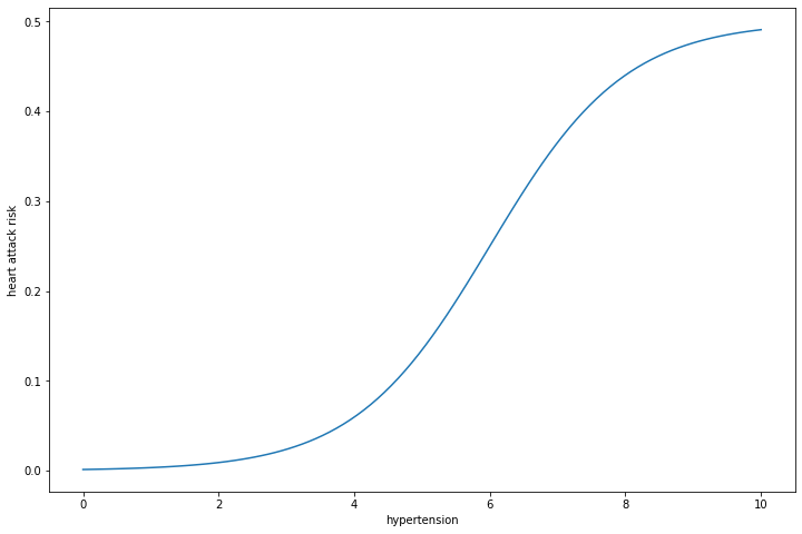
Fact 4. Hypertension is a risk factor for heart attacks
def sigmoid(x):
    return 1 / (1 + np.exp(-x))

def heart_attack_risk(hypertension, heart_attack_proclivity=0.5):
    return heart_attack_proclivity * sigmoid(hypertension - 6)
import matplotlib.pyplot as plt
%matplotlib inline

plt.figure(figsize=(12,8))
xspace = np.linspace(0, 10, 100)
plt.xlabel('hypertension')
plt.ylabel('heart attack risk')
plt.plot(xspace, heart_attack_risk(xspace))
[<matplotlib.lines.Line2D at 0x7fb8b4a2ed60>]
def heart_attack_occured(state, heart_attack_proclivity=0.5):
    return np.random.uniform(0, 1) < heart_attack_risk(state['hypertension'], heart_attack_proclivity)
heart_attack_occured(state)
False
Fact 5. Hypertension and intoxication decay exponentially over time, with a half-life of around 12 hours (24 half-hours)
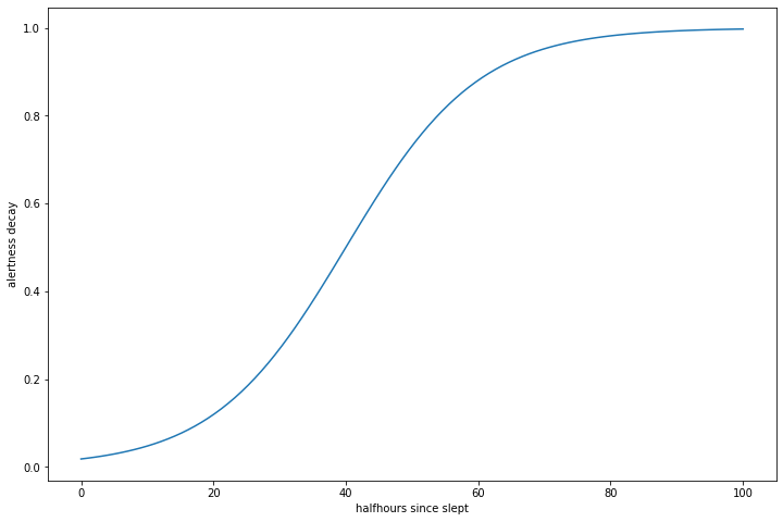
Fact 6. Alertness decays if you haven’t slept for a long time
def alertness_decay(time_since_slept):
    return sigmoid((time_since_slept - 40) / 10)
plt.figure(figsize=(12,8))
xspace = np.linspace(0, 100, 100)
plt.xlabel('halfhours since slept')
plt.ylabel('alertness decay')
plt.plot(xspace, alertness_decay(xspace))
[<matplotlib.lines.Line2D at 0x7fb8ac9c0400>]
decay_rate = 0.97
half_life = decay_rate ** 24
half_life
0.48141722191172337
def half_hour_passed(state):
    state['alertness'] -= alertness_decay(state['time_since_slept'])
    state['hypertension'] = decay_rate * state['hypertension']
    state['intoxication'] = decay_rate * state['intoxication']
    state['time_since_slept'] += 1
    state['time_elapsed'] += 1
half_hour_passed(state)
state
{'alertness': 0.8270396053524154,
 'hypertension': 0.4701967896921894,
 'intoxication': 0.012121832164124767,
 'time_since_slept': 1,
 'time_elapsed': 1,
 'work_done': 0}
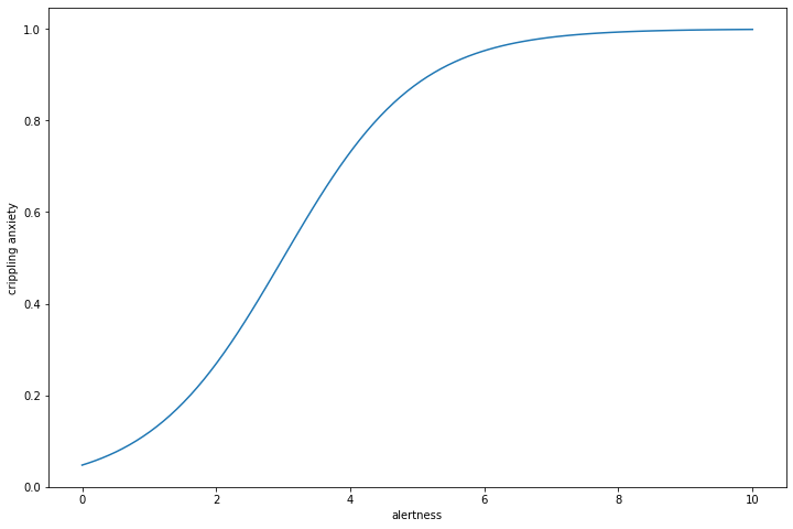
Fact 7. In order to work productively, you have to be alert, but not so alert that crippling anxiety hits
def crippling_anxiety(alertness):
    return sigmoid(alertness - 3)
plt.figure(figsize=(12,8))
xspace = np.linspace(0, 10, 100)
plt.xlabel('alertness')
plt.ylabel('crippling anxiety')
plt.plot(xspace, crippling_anxiety(xspace))
[<matplotlib.lines.Line2D at 0x7fb8ac92e310>]
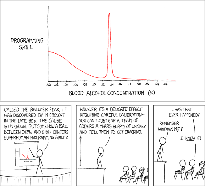
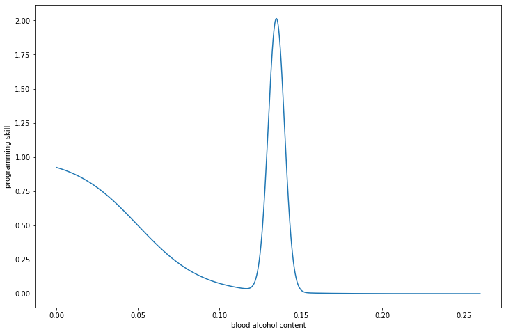
Fiction 8. Relationship between intoxication level and productivity is modelled by the Ballmer function:
def gaussian(x, mu, sig):
    return np.exp(-np.power(x - mu, 2.) / (2 * np.power(sig, 2.)))

def ballmer_function(intoxication):
    return sigmoid((0.05 - intoxication) * 50) + 2 * gaussian(intoxication, 0.135, 0.005)
plt.figure(figsize=(12,8))
xspace = np.linspace(0, 0.26, 1000)
plt.xlabel('blood alcohol content')
plt.ylabel('programming skill')
plt.plot(xspace, ballmer_function(xspace))
[<matplotlib.lines.Line2D at 0x7fb8ac90f7c0>]
def productivity(state):
    p = 1
    p *= state['alertness']
    p *= 1 - crippling_anxiety(state['alertness'])
    p *= ballmer_function(state['intoxication'])
    return p
state
{'alertness': 0.8270396053524154,
 'hypertension': 0.4701967896921894,
 'intoxication': 0.012121832164124767,
 'time_since_slept': 1,
 'time_elapsed': 1,
 'work_done': 0}
productivity(state)
0.645391786501011
def work(state):
    state['work_done'] += productivity(state)
    half_hour_passed(state)
work(state)
state
{'alertness': 0.8071992996183379,
 'hypertension': 0.4560908860014237,
 'intoxication': 0.011758177199201024,
 'time_since_slept': 2,
 'time_elapsed': 2,
 'work_done': 0.645391786501011}
Hopefully, the powers of Reinforcement Learning will help us improve this state!
Writing the environment class
To write own OpenAI gym environment, you have to:
- Create a class that inherits from
gym.Env - Make sure that it has
action_spaceandobservation_spaceattributes defined - Make sure it has
reset(),step(),close()andrender()functions defined. See our exploration of MountainCar above for an intuition on how this functions are supposed to work
Let’s do that, shall we?
First, we need to decide what the action and observation spaces of HeartPole are going to look like.
Every half an hour of working you stop and do one of the following:
- Nothing
- Drink coffee
- Drink beer
- Go to sleep
If you’ve chosen 1-3, you immediately go back to work, if you’ve chosen sleep, you sleep for 16 half-hours and go back to work
def do_nothing(state):
    pass

def sleep(state):
    """Have 16 half-hours of healthy sleep"""
    for hh in range(16):
        half_hour_passed(state)
    wakeup(state)

actions = [do_nothing, drink_coffee, drink_beer, sleep]
So, it is a 4-way discrete action space
heartpole_action_space = gym.spaces.Discrete(len(actions))
As for the observations, we observe the state of the patient, which is the following:
state
{'alertness': 0.8071992996183379,
 'hypertension': 0.4560908860014237,
 'intoxication': 0.011758177199201024,
 'time_since_slept': 2,
 'time_elapsed': 2,
 'work_done': 0.645391786501011}
So, it’s a Box of shape (6,)
observations = ['alertness', 'hypertension', 'intoxication',
                    'time_since_slept', 'time_elapsed', 'work_done']

def make_heartpole_obs_space():
    lower_obs_bound = {
        'alertness': - np.inf,
        'hypertension': 0,
        'intoxication': 0,
        'time_since_slept': 0,
        'time_elapsed': 0,
        'work_done': - np.inf
    }
    higher_obs_bound = {
        'alertness': np.inf,
        'hypertension': np.inf,
        'intoxication': np.inf,
        'time_since_slept': np.inf,
        'time_elapsed': np.inf,
        'work_done': np.inf
    }

    low = np.array([lower_obs_bound[o] for o in observations])
    high = np.array([higher_obs_bound[o] for o in observations])
    shape = (len(observations),)
    return gym.spaces.Box(low,high,shape)
Aaaaaaaaaaand, voila!
class HeartPole(gym.Env):
    def __init__(self, heart_attack_proclivity=0.5, max_steps=1000):
        self.actions = actions
        self.observations = observations
        self.action_space = heartpole_action_space
        self.observation_space = make_heartpole_obs_space()
        self.heart_attack_proclivity = heart_attack_proclivity
        self.log = ''
        self.max_steps = max_steps

    def observation(self):
        return np.array([self.state[o] for o in self.observations])

    def reset(self):
        self.state = {
            'alertness': 0,
            'hypertension': 0,
            'intoxication': 0,
            'time_since_slept': 0,
            'time_elapsed': 0,
            'work_done': 0
        }
        self.steps_left = self.max_steps

        wakeup(self.state)
        return self.observation()

    def step(self, action):
        if self.state['time_elapsed'] == 0:
            old_score = 0
        else:
            old_score = self.state['work_done'] / self.state['time_elapsed']

        # Do selected action
        self.actions[action](self.state)
        self.log += f'Chosen action: {self.actions[action].__name__}\n'

        # Do work
        work(self.state)

        new_score = self.state['work_done'] / self.state['time_elapsed']

        reward = new_score - old_score

        if heart_attack_occured(self.state, self.heart_attack_proclivity):
            self.log += f'HEART ATTACK\n'

            # We would like to avoid this
            reward -= 100

            # A heart attack is like purgatory - painful, but cleansing
            # You can tell I am not a doctor
            self.state['hypertension'] = 0

        self.log += str(self.state) + '\n'

        self.steps_left -= 1
        done = (self.steps_left <= 0)

        return self.observation(), reward, done, {}

    def close(self):
        pass

    def render(self, mode=None):
        print(self.log)
        self.log = ''
Note that most RL algorithms trains in episodes - they take actions in the environment until the done variable becomes true. When it does, the episode is considered to have finished and updates are made to the policy to perform better next episode.
Our HeartPole environment is theoretically infinite - why would you ever stop working? But due to the nature of episode-based training, it is still a good idea to build in an adjustable time limit, like we did with max_steps variable in the code above. We just make sure that the episode length isn’t too short to experience long-term effects. Let’s drink coffee every half an hour and see how soon we get a heart attack:
heartpole = HeartPole()
/home/vadim/.pyenv/versions/3.9.7/lib/python3.9/site-packages/gym/logger.py:34: UserWarning: [33mWARN: Box bound precision lowered by casting to float32[0m
warnings.warn(colorize("%s: %s" % ("WARN", msg % args), "yellow"))
observation = heartpole.reset()
cups = 0

while 'HEART ATTACK' not in heartpole.log:
    observation, reward, done, _ = heartpole.step(1)
    cups += 1

print(cups)
28
28 steps. So we can be quite certain that a 1000 steps long episode is enough to experience long-term effects.
Registering the environment
The only difference left between “official” gym environments and our HeartPole is that bundled environemnts have an id string like CartPole-v0 and can be created with gym.make. If you insist, this too can be rectified. For that you need to put your environment into a Python file and specify the entry point in the format of module:Class.
In the source code attached to this tutorial we have created a package installable with
!pip install heartpole
See “How to upload your python package to PyPi” if you want to learn how to do it
# Making it official
gym.register('HeartPole-v0', entry_point='heartpole:HeartPole')
heartpole = gym.make('HeartPole-v0')
Testing the environment
!pip install stable-baselines3
To test this environment, let us use stable-baselines3 library to build a DQN agent that uses a Q-network with 3 hidden layers of size 16 to solve the HeartPole task
from stable_baselines3 import DQN

model = DQN("MlpPolicy", heartpole, verbose=1, policy_kwargs={'net_arch': [16,16]})
Using cpu device
Wrapping the env with a `Monitor` wrapper
Wrapping the env in a DummyVecEnv.
Time to train our agent! We will be training it for 500 episodes (1000 steps each)
model.learn(total_timesteps=500000, log_interval=10)
----------------------------------
| rollout/            |          |
|    ep_len_mean      | 1e+03    |
|    ep_rew_mean      | -210     |
|    exploration rate | 0.81     |
| time/               |          |
|    episodes         | 10       |
|    fps              | 994      |
|    time_elapsed     | 10       |
|    total timesteps  | 10000    |
----------------------------------
----------------------------------
| rollout/            |          |
|    ep_len_mean      | 1e+03    |
|    ep_rew_mean      | -225     |
|    exploration rate | 0.62     |
| time/               |          |
|    episodes         | 20       |
|    fps              | 768      |
|    time_elapsed     | 26       |
|    total timesteps  | 20000    |
----------------------------------
----------------------------------
| rollout/            |          |
|    ep_len_mean      | 1e+03    |
|    ep_rew_mean      | -227     |
|    exploration rate | 0.43     |
| time/               |          |
|    episodes         | 30       |
|    fps              | 632      |
|    time_elapsed     | 47       |
|    total timesteps  | 30000    |
----------------------------------
----------------------------------
| rollout/            |          |
|    ep_len_mean      | 1e+03    |
|    ep_rew_mean      | -225     |
|    exploration rate | 0.24     |
| time/               |          |
|    episodes         | 40       |
|    fps              | 542      |
|    time_elapsed     | 73       |
|    total timesteps  | 40000    |
----------------------------------
----------------------------------
| rollout/            |          |
|    ep_len_mean      | 1e+03    |
|    ep_rew_mean      | -232     |
|    exploration rate | 0.05     |
| time/               |          |
|    episodes         | 50       |
|    fps              | 470      |
|    time_elapsed     | 106      |
|    total timesteps  | 50000    |
----------------------------------
We have an agent! Let us see how well it works.
from stable_baselines3.common.evaluation import evaluate_policy
mean_reward, std_reward = evaluate_policy(model, heartpole, n_eval_episodes=5)
print(f'Reward per episode {mean_reward}±{std_reward}')
Reward per episode -2209.6243209284276±303.20949050899924
Homework
Make HeartPole-v1! Add cannabis some new actions that can modify your health and productivity!
Acknowledgements
If you’re an EU taxpayer, you are probably paying for the writing of this post. Unsubscribe requests are handled by your local libertarian party. If you’re Marharyta Beraziuk, thanks for sending me that cannabis paper.