Neurogenetic optimization

Let me start this essay, as one does on the internet, by polarising my audience

But what if I told you that the Montecchi and Cappelletti of gradient free optimization work suprisingly well in tandem?

Background: gradient-free optimization

Consider the task of finding the minimum of a function without any access to it’s derivative:

Here’s the function:

\[ O(x) = sin x + sin 10x - 0.01x^2 \]

Yes, the mathematically gifted members of the audeince have probably already derived the gradient of the function analytically. However, a lot of functions we would like to optimize in real life (phone battery life, travel time, QALYs, profits) don’t have a handy formula attached. So, for the sake of developing a useful methodology, we treat \(O(x)\) as fully opaque: the only way to learn something about \(O(x)\) is to query the values of \(O(x)\) for some \(x\)s.

This function can also be represented in Python as

import numpy as np

def reward_f(x):
    return np.sin(x) + np.sin(x * 10) - 0.01 * x ** 2

and visualised

min_x = -10
max_x = 10

import matplotlib.pyplot as plt
import seaborn as sns
sns.set_theme(style="darkgrid")

plot_x = np.linspace(min_x, max_x, 1000)
plot_y = reward_f(plot_x)

sns.lineplot(x=plot_x, y=plot_y)

<AxesSubplot:>

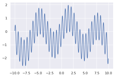
The goal is to find \(\arg\max_x O(x)\)

Evolutionary approach

Start with an intitial population of 2 instances of \(x\)

xs = [min_x, max_x]
rs = [reward_f(min_x), reward_f(max_x)]
rs_exp = [np.exp(reward_f(min_x)), np.exp(reward_f(max_x))]

At every iteration of the evolutionary algorithm, draw \(x_1\) and \(x_2\) from the exponential reward distribution:

\[ p(x) \sim e^{O(x)} \]

And add \(\frac{x_1 + x_2}{2}\) to the population

def genetic_step():
    parent1, parent2 = np.random.choice(xs, size=2, p=rs_exp/np.sum(rs_exp))
    new_x = (parent1 + parent2) / 2
    new_r = reward_f(new_x)
    
    xs.append(new_x)
    rs.append(new_r)
    rs_exp.append(np.exp(new_r))

Repeat for 10000 iterations

from tqdm.notebook import tqdm

for _ in tqdm(range(10000), leave=False):
    genetic_step()

From the resulting population of 10002 pick \(x\) with the maximal \(O(x)\)

best_idx = np.argmax(rs)

By generating new solutions as modifications of existing successful solutions we focus the search on the most promising part of the search space. The visualisation below shows the history of the search, note that the darker colored points were added to the population after the light colored ones. The cross denotes the final solution.

sns.lineplot(x=plot_x, y=plot_y)
sns.scatterplot(x=xs, y=rs, hue=range(len(xs)))
sns.scatterplot(x=[xs[best_idx]], y=[rs[best_idx]], marker='x', s=300)

<AxesSubplot:>

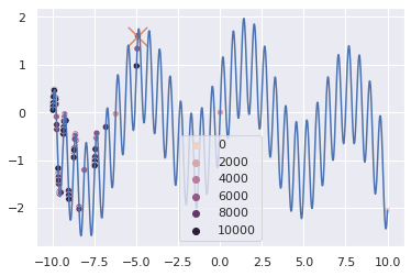
One can see that 10000 iterations were not enough to find the highest peak, although the one we finally found is close. Most of the iterations were spent navigating the far left part of the search space. The right half of the search space remained unexplored - the rightmost solution \(x_\text{right}\) has an \(O(x_\text{right})=-2\) which means it’s almost never drawn from \(p(x)\). This could be mitigated by a number of tricks, for instance, adding a temperature parameter to \(p(x)\):

\[ p_t(x) \sim e^{tO(x)} \]

but the issue is fundamenal to evolutionary algorithms - a few unrepresentative examples can erroneously exclude a large part of the search space.

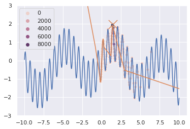
Neural Actor-Critic approach

In the deep learning approach we train a critic neural network \(\hat{O}_{\phi}(x)\) to mimic \(O(x)\) as closely as possible. Then all we need is a second neural network that represents a probability distribution of \(x\)s that have a high \(O(x)\) and sample from it. It is called the actor network, \(x_{\phi}(z)\), representing a mapping from the normal distribution to the distribution of points with high \(O(x)\). See actor-critic methods in Reinforcement Learning.

import torch
from torch import nn

actor = nn.Sequential(
    nn.Linear(1, 10),
    nn.ReLU(),
    nn.Linear(10, 10),
    nn.ReLU(),
    nn.Linear(10, 1)
)

actor_opt = torch.optim.Adam(actor.parameters())

critic = nn.Sequential(
    nn.Linear(1, 10),
    nn.ReLU(),
    nn.Linear(10, 10),
    nn.ReLU(),
    nn.Linear(10, 1)
)
critic_opt = torch.optim.Adam(critic.parameters())

We start with an empty population

xs = []
rs = []
rs_exp = []

At every step, we sample \(z\) from \(N(0,1)\), add \(x_{\phi}(z)\) to the population and update both \(\hat{O}_{\phi}(x)\) and \(x_{\phi}(z)\).

def neural_step():
    z = torch.normal(mean=torch.tensor([0.0]),
                     std=torch.tensor([1.0]))
    x = actor(z).detach().numpy()[0]
    r = reward_f(x)
    
    xs.append(x)
    rs.append(r)
    rs_exp.append(np.exp(r))
    
    critic_loss = (critic(torch.tensor(xs).float().reshape(-1,1)) 
                        - torch.tensor(rs).float().reshape(-1,1)) ** 2
    critic_loss = critic_loss.sum()
    
    critic_loss.backward(retain_graph=True)
    critic_opt.step()
    critic_opt.zero_grad()
    
    z = torch.normal(mean=torch.zeros(10),
                     std=torch.ones(10))
    z = z.reshape(-1, 1)
    actor_loss = - critic(actor(z)).sum()
    actor_loss.backward()
    actor_opt.step()
    actor_opt.zero_grad()

for _ in tqdm(range(10000), leave=False):
    neural_step()
    
best_idx = np.argmax(rs)

  0%|          | 0/10000 [00:00<?, ?it/s]

xs = np.array(xs)
rs = np.array(rs)
critic_rs = critic(torch.tensor(plot_x.reshape(-1, 1).astype('float32'))).detach().numpy().reshape(-1)

sns.lineplot(x=plot_x, y=plot_y)
sns.scatterplot(x=xs, y=rs, hue=range(len(xs)))
sns.scatterplot(x=[xs[best_idx]], y=[rs[best_idx]], marker='x', s=300)
sns.lineplot(x=plot_x, y=critic_rs)
plt.ylim(-3, 3)

(-3.0, 3.0)

Neurogenetic approach

xs = []
rs = []
rs_exp = []

neural_step()
for _ in tqdm(range(10000), leave=False):
    neural_step()
    genetic_step()
    
best_idx = np.argmax(rs)

  0%|          | 0/10000 [00:00<?, ?it/s]

sns.lineplot(x=plot_x, y=plot_y)
sns.scatterplot(x=xs, y=rs, hue=range(len(xs)))
sns.scatterplot(x=[xs[best_idx]], y=[rs[best_idx]], marker='x', s=300)
sns.lineplot(x=plot_x, y=critic_rs)
plt.ylim(-3, 3)

(-3.0, 3.0)

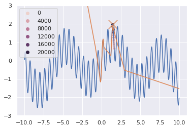
One can see that in the hybrid neural-genetic mode, the search process zeros in on the maximum really fast and finds it within 4000 iterations, faster than both pure neural and pure genetic approaches

Going beyond this simple example

A simple \(O(x):R \rightarrow R\) was used to make the illustration as clear and simple as possible. The principle can be applied to any gradient-free optimization task, including complex search spaces where the domain of \(O(x)\) is images, texts or, say, trading strategies. See this paper by a truly brilliant group of authors applying it to the task of program synthesis

Confessions

This work is taxpayer funded